A demonstration of TDOA multilateration

Yesterday, a thread popped up on r/Albuquerque where users attempted to identify the source of a loud explosion in the early morning. A few individuals provided their locations and timestamps at which their surveillance cameras detected the sound. I thought I could use this information to pinpoint its source using multilateration.

What is multilateration?

Multilateration is the process by which an energy source can be located based on observations of the energy at different locations. The energy can be a light, radio, acoustic, or seismic wave; the time the wave takes to travel to each observer allows us to solve a system of equations to identify the unknown source. The process works mostly the same for all types of waves, just the speed of transmission varies. In this case, we’ll be using acoustic energy, which is fairly resilient to timing errors. Sound takes about five seconds to travel one mile, so even if the timestamps are not accurate we can get fairly close to the source.

Multilateration has many real-world applications, for example the acoustic form we’re studying today is used in law enforcement and defense, and its radio counterparts are used for aircraft tracking and navigation. Its wide range applicability has resulted in this being a very well-studied problem. However, one might expect it to be difficult to understand. In this article, we’ll look at the mathematics of multilateration and find in it a surprising simplicity.

How does it work?

Since we want to locate the event based on the differences in times of detection, what we’re doing is actually TDOA (time difference of arrival) multilateration. For simplicity, we’ll assume a flat Earth and attempt to solve the problem in the Cartesian plane. If we know the difference in arrival time between two points, we can describe the possible locations of the event as a hyperbola. In fact, one of the ways a hyperbola can be defined is as the set of points which have a fixed distance between two fixed points.

The hyperbola we’re interested in can be described as

$$\sqrt{(x - x_1)^2 + (y - y_1)^2} - \sqrt{(x - x_0)^2 + (y - y_0)^2} - v(t_1 - t_0) = 0$$

where $x_0, y_0$ is the position of the first observer, $t_0$ is its observation time, $x_1, y_1, t_1$ are those parameters of the second observer, and $v$ is the propagation speed of the wave we’re interested in.

It’s easy to identify the two instances of the Cartesian distance formula here. In fact, the first square root represents distance between the event and the second observer, and the second gives the distance between the event and the first observer. Therefore, the equation can easily be parsed as providing the set of points that have distance $v(t_1 - t_0)$ from both observers. We’ll refer to this quantity proportional to the difference in arrival times as a pseudodistance.

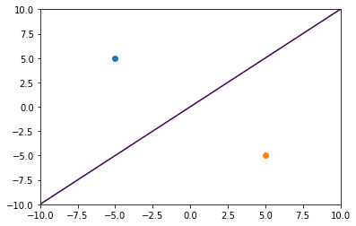
For example, consider the case where the two observers notice the event at the same time. We can intuit that we should observe a line.

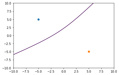
If we were to determine that the TDOA between the observers correlates to a pseudodistance of 3, then we can begin to observe the development of the hyperbolic curvature. In this case, we’ve made the event closer to the top-left observer.

By adding a third observer, we can draw a second hyperbola.

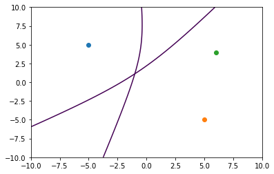
In this case, we’ve set a pseudodistance of 2 between the first and third observers’ observations. The intersection between the two hyperbolae gives us a solution indicating the source of the event.

A practical example

To protect the privacy of the users who contributed, we’ll walk through a fake example instead of the one discussed on Reddit. I’ve generated some points in the middle of the desert with a synthetic event. We’ll be using Python code to solve the multilateration.

First, let’s define the observation locations and timestamps.

measurements = [
    [34.888, -103.826, 0.0],
    [34.931, -103.805, 0.6],
    [34.921, -103.781, 2.5]
]

This is simply a list of the latitudes and longitudes of the observers, with timestamps representing the TDOA from the first observation in seconds.

Now that we have input data, the first step is to convert the geodetic coordinates to something we can work with more easily. To keep things simple, we’ll go to ENU (east-north-up) coordinates centered at the first observer, and discard the up component to keep things in the plane.

import pymap3d as pm

lat0, lon0, t0 = measurements[0]
for i in range(len(measurements)):
    lat, lon, t = measurements[i]
    e, n, _ = pm.geodetic2enu(lat, lon, 0, lat0, lon0, 0)
    measurements[i] = [e, n, t]

After this, measurements has the content [[0.0, 0.0, 0.0], [1918.6593908214895, 4770.574154674195, 0.6], [4111.911492926018, 3661.9046769939555, 2.5]], where each entry gives us the distance east, north from the first observer (in meters) and its time of observation.

Since we’re working with meters and seconds, let’s define the speed of sound with respect to those units:

speed = 343. # m/s

Next, we need to figure out how to define and solve the system of hyperbolic equations. I’m going to use scipy’s least-squares solver so we’ll specify the system in a way that we can use with it.

import numpy as np

def functions(x0, y0, x1, y1, x2, y2, d01, d02, d12):
    """ Given observers at (x0, y0), (x1, y1), (x2, y2) and TDOA between observers d01, d02, d12, this closure
        returns a function that evaluates the system of three hyperbolae for given event x, y.
    """
    def fn(args):
        x, y = args
        a = np.sqrt(np.power(x - x1, 2.) + np.power(y - y1, 2.)) - np.sqrt(np.power(x - x0, 2.) + np.power(y - y0, 2.)) - d01
        b = np.sqrt(np.power(x - x2, 2.) + np.power(y - y2, 2.)) - np.sqrt(np.power(x - x0, 2.) + np.power(y - y0, 2.)) - d02
        c = np.sqrt(np.power(x - x2, 2.) + np.power(y - y2, 2.)) - np.sqrt(np.power(x - x1, 2.) + np.power(y - y1, 2.)) - d12
        return [a, b, c]
    return fn

We’ve added the third hyperbola which represents the TDOA between the second and third observers, in addition to the two we have already discussed.

To help out the solver a bit, we can also specify the Jacobian matrix of this system. This is just a collection of the partial derivatives of each function with respect to each independent variable.

def jacobian(x0, y0, x1, y1, x2, y2, d01, d02, d12):
    def fn(args):
        x, y = args
        adx = (x - x1) / np.sqrt(np.power(x - x1, 2.) + np.power(y - y1, 2.)) - (x - x0) / np.sqrt(np.power(x - x0, 2.) + np.power(y - y0, 2.))
        bdx = (x - x2) / np.sqrt(np.power(x - x2, 2.) + np.power(y - y2, 2.)) - (x - x0) / np.sqrt(np.power(x - x0, 2.) + np.power(y - y0, 2.))
        cdx = (x - x2) / np.sqrt(np.power(x - x2, 2.) + np.power(y - y2, 2.)) - (x - x1) / np.sqrt(np.power(x - x1, 2.) + np.power(y - y1, 2.))
        ady = (y - y1) / np.sqrt(np.power(x - x1, 2.) + np.power(y - y1, 2.)) - (y - y0) / np.sqrt(np.power(x - x0, 2.) + np.power(y - y0, 2.))
        bdy = (y - y2) / np.sqrt(np.power(x - x2, 2.) + np.power(y - y2, 2.)) - (y - y0) / np.sqrt(np.power(x - x0, 2.) + np.power(y - y0, 2.))
        cdy = (y - y2) / np.sqrt(np.power(x - x2, 2.) + np.power(y - y2, 2.)) - (y - y1) / np.sqrt(np.power(x - x1, 2.) + np.power(y - y1, 2.))

        return [
            [adx, ady],
            [bdx, bdy],
            [cdx, cdy]
        ]
    return fn

As a last preparation before solving, we can provide an initial guess for the location of the event. We’ll just use the average of the three observer locations. This helps avoid issues with points for which the function is not well-defined.

xp = np.mean([x for x,y,t in measurements])
yp = np.mean([y for x,y,t in measurements])

Finally, we can run the solver:

import scipy.optimize as opt

x0, y0, t0 = measurements[0]
x1, y1, t1 = measurements[1]
x2, y2, t2 = measurements[2]

F = functions(x0, y0, x1, y1, x2, y2, (t1 - t0) * speed, (t2 - t0) * speed, (t2 - t1) * speed)
J = jacobian(x0, y0, x1, y1, x2, y2, (t1 - t0) * speed, (t2 - t0) * speed, (t2 - t1) * speed)

x, y, _ = opt.leastsq(F, x0=[xp, yp], Dfun=J)

This gives us a solution of 1109.306162, 2213.711852 in ENU space relative to the first receiver. We can convert that back to geodetic coordinates to make it more useful:

lat, lon, _ = pm.enu2geodetic(x, y, 0, lat0, lon0, 0)

We have now determined the location of the event to be 34.907954, -103.813862.

The system of hyperbolae and the solution can be visualized:

import matplotlib.pyplot as plt

# Create reasonable x, y bounds for visualization
max_x = max(x0, x1, x2, x)
min_x = min(x0, x1, x2, x)
range_x = max_x - min_x
min_x -= range_x * .2
max_x += range_x * .2

max_y = max(y0, y1, y2, y)
min_y = min(y0, y1, y2, y)
range_y = max_y - min_y
min_y -= range_y * .2
max_y += range_y * .2

# Create a grid of input coordinates
xs = np.linspace(min_x, max_x, 100)
ys = np.linspace(min_y, max_y, 100)
xs, ys = np.meshgrid(xs, ys)

# Evaluate the system across the grid
A, B, C = F((xs, ys, np.zeros(xs.shape)))

# Plot the results
plt.scatter(x0, y0, color='r')
plt.scatter(x1, y1, color='g')
plt.scatter(x2, y2, color='b')
plt.scatter(x, y, color='k')
plt.contour(xs, ys, A, [0], colors='y')
plt.contour(xs, ys, B, [0], colors='m')
plt.contour(xs, ys, C, [0], colors='c')
plt.show()

We’ve somewhat abused matplotlib’s contour function here by evaluating the grid and plotting the contour for just the zeros of the function. The result is the following:

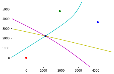
This allows us to visually confirm that the reported solution is at the intersection of the hyperbolae.

We can also derive each observer’s distance from the event and the time-of-flight of the energy.

d0 = np.sqrt(np.power(x - x0, 2.) + np.power(y - y0, 2.))
d1 = np.sqrt(np.power(x - x1, 2.) + np.power(y - y1, 2.))
d2 = np.sqrt(np.power(x - x2, 2.) + np.power(y - y2, 2.))
t0 = d0 / speed
t1 = d1 / speed
t2 = d2 / speed

This lets us know that the distances from each observer are 2476 m, 2682 m, and 3334 m respectively; the corresponding times of flight are 7.2 s, 7.8 s, and 9.7 s. This confirms the TDOAs of 0.6 s and 2.5 s that we provided as input.

We can also use this information to plot circles around each observer, which gives us a more traditional triangulation diagram, though in this case it is synthetic.

def circle(cx, cy, r):
    def fn(x, y):
        return np.sqrt(np.power(x - cx, 2.) + np.power(y - cy, 2.)) - r
    return fn

c0 = circle(x0, y0, d0)
c1 = circle(x1, y1, d1)
c2 = circle(x2, y2, d2)

plt.scatter(x0, y0, color='r')
plt.scatter(x1, y1, color='g')
plt.scatter(x2, y2, color='b')
plt.scatter(x, y, color='k')

plt.contour(xs, ys, c0(xs, ys), [0], colors='r')
plt.contour(xs, ys, c1(xs, ys), [0], colors='g')
plt.contour(xs, ys, c2(xs, ys), [0], colors='b')
plt.show()

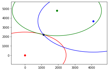
We can see that the intersection of the circles also lies at the event.

Conclusion

I apologize that this is only a shallow overview of multilateration (mostly because I only have a shallow understanding) and for the simplicity of the example. However, two-dimensional multilateration still provides the groundwork for the three-dimensional applications I mentioned earlier. In those cases, we’re solving for the intersection of hyperboloids instead of hyperbolae, for which at least four observers are required. In applications like low-frequency radio waves, the curvature of the earth also needs to be considered, making the mathematics much more complicated. In seismology, variations in Earth’s density also introduce additional complexity. I like the acoustic example given here because of its simplicity, and hopefully some readers found the exercise interesting nonetheless.