Generating terrain meshes for 3D printing

A while back, I thought 3D printed models of the local terrain might be a cool gift idea. To make this a reality, I have implemented a simple Python utility to convert publicly-available terrain data into a format suitable for 3D printing.

Most 3D printers expect STL models, which define a solid in terms of vertices in 3D Cartesian space and faces (triangles) which connect them. However, terrain models are typically distributed as rasters of heights indexed by latitudes and longitudes. Fortunately, libraries exist to convert latitude, longitude, altitude tuples to standardized Cartesian coordinates. However, some additional massaging of the data is required.

If you’re interested in the details of this process, read on. Otherwise, the project is available on Github for immediate use, without you needing to worry about it.

Getting the data

Before we can start, we need to find terrain data to work with. Fortunately, NASA has been kind enough to make its SRTMGL3 dataset public, which gives us fairly high-quality terrain data for (mostly) the entire world. I don’t know how the radar magic that they used to create these models works, but fortunately the form they are distributed in is fairly easy to work with.

Each raster, or “granule,” covers a square measuring 1 degree of latitude and 1 degree of longitude. At the 3 arcsecond resolution we’ll be using, this gives us a raster of 1201 by 1201 pixels. The data is stored as a matrix of big-endian signed shorts without any sort of metadata, and thus we can read it with a simple one-liner in numpy:

altitudes = np.fromfile(filename, dtype='>i2', count=1201 * 1201).reshape((1201, 1201))

Now we’ve got a matrix representing the altitudes associated with the latitude and longitude of each pixel. The latitudes and longitudes themselves are determined by the pixel coordinates as well as the filename. The filename itself reveals the latitude and longitude of the bottom-left (southwest) corner of the raster; each pixel is 3 arcseconds by 3 arcseconds in size.

Again, we can use a few simple numpy incantations to give us arrays of latitudes and longitudes that we can index in parallel with the altitudes we extracted:

lats = np.linspace(north_latitude, south_latitude, num_rows, False)
lons = np.linspace(west_longitude, east_longitude, num_cols, False)
longrid, latgrid = np.meshgrid(lons, lats)

If the region we want to 3D print lies entirely within one SRTM granule, this is almost all we have to do. However, we must cover an edge case where the target area spans more than a single raster.

Merging granules and extracting the target area

Unless we’re 3D printing an area that itself spans more than 1 square degree (which I wouldn’t recommend due to the limited visibility of terrain detail at this size), the worst case scenario we will encounter requires us to merge four adjacent rasters.

If we determine that the requested area spans more than one raster, we simply load all of the required rasters and merge them as follows:

merged = np.block(blocks)

where blocks is a 2D list representing the physical layout of the rasters we are merging, and each element is a loaded raster. It is important to note that you must trim off the first row and last column in this step, as they are overlapped with the adjacent granules.

Now that we have aggregated the granules of interest, we can extract the region we want:

r0 = 1200 - int((north - floor(north)) * 1200)
c0 = int((west - floor(west)) * 1200)
rows = int((north - south) * 3600 // 3 + 1)
cols = int((east - west) * 3600 // 3 + 1)
result = merged[r0:r0+rows, c0:c0+cols]

At this point, we can also apply a scaling factor to the altitudes in order to exaggerate the altitudes and make the 3D printed result more interesting to look at.

Converting to Cartesian coordinates

At this stage, we have extracted vectors of altitudes, latitudes, and longitudes corresponding to the data we wish to 3D print. However, we must combine these three parallel vectors into a coherent set of 3D vertices.

Latitudes and longitudes are ellipsoidal coordinates that give us a point on the surface of the Earth, as opposed to a point on a plane. While it is reasonable to exploit the local linearity of the surface of the ellipsoid and use simple scaling factors to generate a set of vertices above a fixed plane, I actually found it easier to use the “real” conversion between ellipsoidal and Cartesian coordinates for this step.

I found that the most convenient coordinate system to use was ECEF, or Earth Centered Earth Fixed. This is a simple 3D Cartesian system where the origin (0, 0, 0) is located at the center of the Earth, and vectors are expressed in meters relative to this.

I used the Python library pyproj to perform the conversion as follows:

ECEF = pyproj.Proj(proj='geocent', ellps='WGS84', datum='WGS84')
LLA = pyproj.Proj(proj='latlong', ellps='WGS84', datum='WGS84')
x, y, z = pyproj.transform(LLA, ECEF, longrid, latgrid, altitudes, radians=False)

Now we have three parallel arrays representing our vertices.

Correcting orientation, positioning, and scale

Unfortunately, the ellipsoidal to ECEF conversion essentially gives us a patch somewhere on the surface of the Earth, and thus it is not oriented correctly for 3D printing. To correct the orientation, I exploited some facts about the geometry of the Earth ellipsoid the ECEF coordinate system.

First, we must ensure that the model is “right side up.” We can use an ellipsoidal normal vector to approximate “up” and rotate our vertices such that this vector aligns with the z-axis. To avoid re-learning geometry, I simply used pyproj to find the axis:

def get_axis(lat0, lon0, alt0, lat1, lon1, alt1):
    v0 = pyproj.transform(LLA, ECEF, lon0, lat0, alt0, radians=False)
    v1 = pyproj.transform(LLA, ECEF, lon1, lat1, alt1, radians=False)
    v = np.array(v1) - np.array(v0)
    return v

z_axis = get_axis(center_lat, center_lon, 0., center_lat, center_lon, 1000.)

I did something similar to align the north and south edges of the model relative to the x axis:

x_axis = get_axis(south, west, 0., south, east, 0.)

Next, we can generate rotation matrices and use the Scipy spatial library to perform the rotation:

def get_rotation(A, B):
    au = A / np.linalg.norm(A)
    bu = B / np.linalg.norm(B)
    R = np.array([[bu[0]*au[0], bu[0]*au[1], bu[0]*au[2]],
                  [bu[1]*au[0], bu[1]*au[1], bu[1]*au[2]],
                  [bu[2]*au[0], bu[2]*au[1], bu[2]*au[2]]])
    return scipy.spatial.transform.Rotation.from_dcm(R)

r0 = get_rotation(z_axis, [1., 0., 0.])
r1 = get_rotation(r0.apply(x_axis), [1., 0., 0.])
r = r1 * r0
vertices = r.apply(vertices)

Our vertices are now oriented above the x-y plane in a way that kind of makes sense. However, the data is still “life size” and must be scaled down. First, we must center them around the origin in x-y space:

x, _, z = np.mean(vertices, axis=0)
_, y, _ = vertices.min(axis=0)
vertices = np.subtract(vertices, [x, y, z])

Now, they can be scaled:

vertices = vertices * scaling_factor

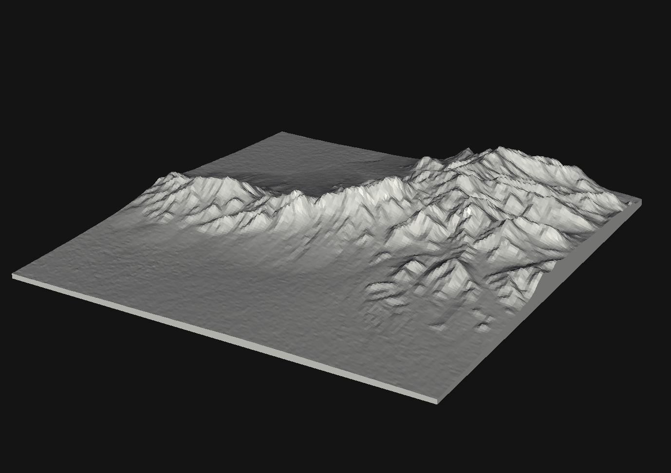
The last step is now to create the faces connecting these vertices, and our 3D model will be complete.

Creating the solid

Despite the amount of math we saw in the previous section, I found this step to be the most difficult. Building faces over the vertices along the “top” of the model, where the terrain is, was relatively straightforward; however, making the model solid at the sides and bottom was a bit trickier.

At this point, it’s been long enough since I wrote the code that I don’t remember what exactly I was doing. To make things worse, it would appear that I didn’t write any comments. Therefore, all I can do is link the relevant section of code and wish you the best, if you wish to attempt understanding it.

Exporting the mesh

At this point, we are ready to export our mesh as an STL file. This is yet another relatively straightforward file format, consisting of a mostly-useless header and a list of vertices that form each face. Each face also has some optional auxiliary information and a normal vector, however I found that populating this was unnecessary. Using Python’s builtin struct module, we can easily pack our floating-point coordinates into the file:

fh.write(b'\0' * 80)
fh.write(struct.pack('<I', len(triangles)))
for a, b, c in triangles:
    fh.write(struct.pack('<fff', 0, 0, 0))
    fh.write(struct.pack('<fff', *vertices[a]))
    fh.write(struct.pack('<fff', *vertices[b]))
    fh.write(struct.pack('<fff', *vertices[c]))
    fh.write(struct.pack('<H', 0))

Now we’re finally ready to print. However, not having my own 3D printer, I ended up sending the model over to Shapeways. It turned out pretty great:

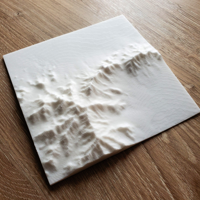
Again, the code is available here on Github: https://github.com/tmick0/topostl